On Rising Rates: Fixed Income Investing

In the first post of this three part series, On Rising Interest Rates, we shared our thoughts on the current and expected interest rate environments. The current outlooks for US economic growth and inflation are both currently low. Regarding inflation expectations, there is an interesting paper on “structural traps” (written in 2004 and found here) that provides some explanation on why quantitative easing has not generated higher inflation expectations. The argument in the paper may explain why inflation expectations collapse when the Fed telegraphs their intention to taper. Combining that with the fact that real growth has not been as strong, the outlook for nominal growth remains muted. Though we believe that rates will rise going forward, the size of those movements may not be as pronounced as the current forward rates imply. However, this “sideways” movement in rates will be more volatile as the Fed has stressed that asset purchases remain dependent on the economic outlook.

In this post, we will discuss the effects of rising interest rates on fixed income instruments. We will focus on the technical mechanics of the yield curve along with economic fundamentals and monetary policy. We think it is important to understand this particular aspect of fixed income investing. Importantly, we do not focus on credit risk during this series of posts. In the final post of this series, we will share our thoughts on how best to structure a fixed income portfolio in such an environment, especially from a multi-manager (as opposed to individual bond) point of view.

Roll Down Math

The total return of a fixed income instrument can be decomposed into two components:

1. Income (coupon/interest payments) and
   
2. Price (capital gain/loss when a bond matures, is sold or called).
   

For this particular discussion, we are interested in one subcomponent of price return: roll down return. Roll down occurs as a bond with a fixed maturity date gets closer to maturity. In a normal market environment, yields tend to decline as the maturity date gets closer and prices tend to rise as investors price the bond relative to a shorter maturity date on the yield curve.

Roll Down — Example

For simplicity, we will use zero-coupon Treasury bonds, which are priced exactly at their respective present values. On October 11^th, 2013, 10-yr and a 5-yr zero-coupon Treasury bonds are purchased at yields of 2.69% and 1.42%, respectively. We will assume that the forward curves accurately reflect the level of future yields. The yield paths are represented by the red and orange dots on the chart below. Please note that the intermediate years’ yield is estimated using linear interpolation.

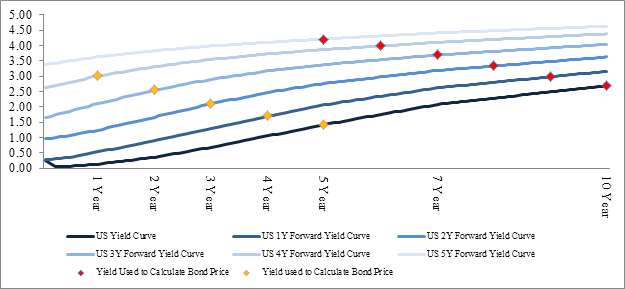
The chart above suggests that over the next 5 years, from the day of investment, yields will keep increasing. We will calculate the price of the bond per $100 par value using the following formula:

Price = (100/((1+yield)^maturity)

The results are shown in the table below.

Several caveats/observations from the above exercise:

• Trading costs and premiums/discounts have not been factored in. This example applies to the purchase of individual bonds. As such, we will present a modified example that considers the purchase of duration managed funds below.
  
• Despite having a theoretically higher return, the 10-yr bond underperforms the 5-yr bond. This result is due to the steepness of the yield curve. On a 5-yr time horizon, the steepest part of the curve occurs at a duration of 3-4 years.
  

Modified Example Number 1

As we noted above, and based on a majority of OFA’s client base, we will modify the exercise to consider an investment in duration managed funds. Suppose that 10-yr and 5-yr zero-coupon Treasury bonds are purchased. Exactly one year from the date of purchase, the bonds are sold and the cash proceeds are used to purchase 10-yr and 5-yr zero-coupon Treasury bonds. In a way, Treasury bond portfolios with an average duration of 9.5 and 4.5 years, respectively, are created. Please refer to the chart below for the estimated yield paths. Again, we will assume that the forward curves accurately reflect the level of future yields. The table following the charts presents the results of the exercise.

The results of the modified example closely mimic the first exercise, suggesting that there are multiple approaches to manage your fixed income exposure during a rising rate environment. We will discuss these strategies using some historical information in the next post.

“The Path of Zero Return”

While loss of principal would imply a negative credit event, we have been faced with considering circumstances in which holding a bond/bond portfolio would produce zero return. In this example, we will consider “the path of zero return”. Using the zero-coupon 10-yr Treasury yielding 2.70% as an example, in order for an investment in the bond to have a 0% return three years from now, the 7-year yield needs to be at 3.88% (the forward curve suggests that the 3 year forward 7-yr yield as of September 9^th, 2013 stands at 3.58%). For that same bond to have a 0% return five years from now, the 5-year yield needs to stand at 5.47% (the forward curve suggests 5-year forward 5-yr yield at 4.07%). This calculation can be done quickly by setting the price of different maturities equal to each other. In the chart below, we give a simple depiction of the “path of zero return”.

The chart above indicates that rates would have to move up very quickly and significantly in order for negative returns to be generated over three and five-year time periods. The current forward curves imply that returns may closely mirror the yields, however, in the long-run, the theoretical zero-return yield level will not be reached.

The Fed’s zero interest rate policy and asset purchase program are designed to stimulate economic growth. In so doing, yields have been suppressed. Given that economic fundamentals remain muted (low growth with deflationary/low inflation pressures), we believe that an accommodative monetary policy stance will remain in place for some time. However, it is prudent to think about the possibility of rising rates as well as the impact such policy has had, and will have, on the shape of the yield curve. This post shows that the magnitude and speed of interest rate moves, as well as time horizon, are important components of fixed income return. If the rising rates scenario implied by the forward rates were to materialize, yield curve technicals and time will provide a good hedge. In the final post, we will discuss some implementable ideas.

Unless otherwise specified, all charts and data points are as of 9/30/2013
Source: FactSet Research Systems